Process Capability Analysis Cp, Cpk, Pp, Ppk - A Guide
01. What is Process Capability Analysis?
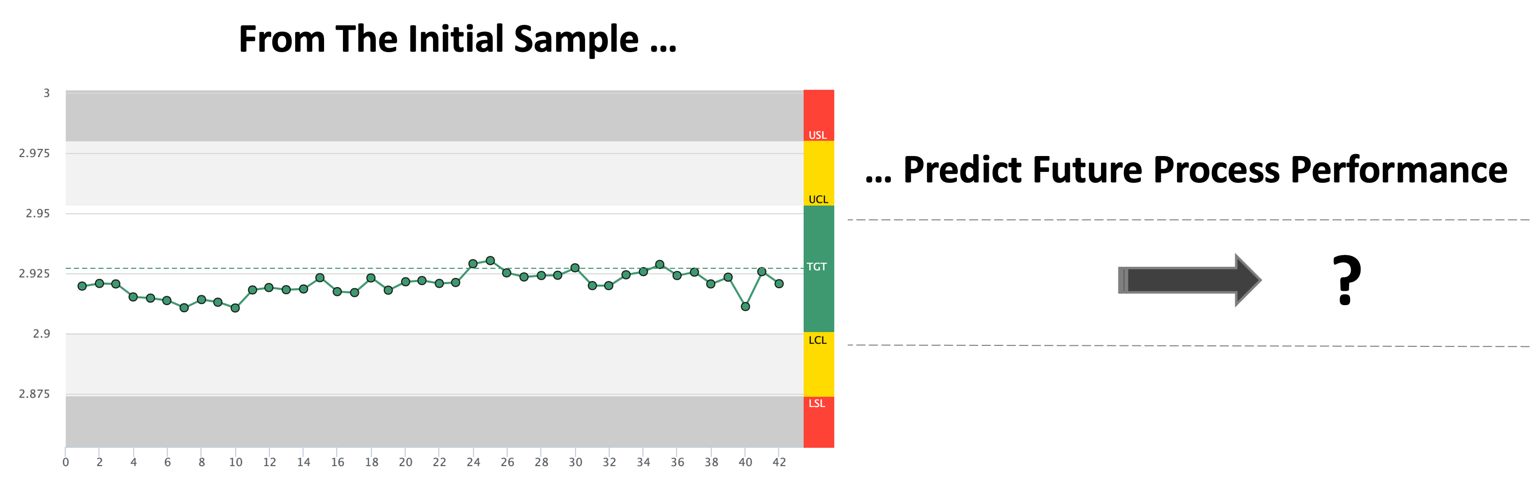
A process capability study uses data from an initial run of parts to predict whether a manufacturing process can repeatably produce parts that meet specifications.
Think of it as being similar to a forecast. You will take some historical data, and extrapolate out to the future to answer the question "can I rely on this process to deliver good parts?".
Your customers may require a process capability study as part of a PPAP. They will do this to ensure that your manufacturing processes are capable of consistently producing good parts.
02. The Basic Concept
When the manufacturing process is being defined, your goal is to ensure that the parts produced fall within the Upper and Lower Specification Limits (USL, LSL). Process Capability measures how consistently a manufacturing process can produce parts within specifications.
The basic idea is very simple. You want your manufacturing process to:
(1) be centered over the Nominal desired by the design engineer, and
(2) with a spread narrower than the specification width.
Cp measures whether the process spread is narrower than the specification width
Cpk measures both the centering of the process as well as the spread of the process relative to the specification width

03. The Basic Calculations
Before we get into the detailed statistical calculations, let's review the high-level steps:
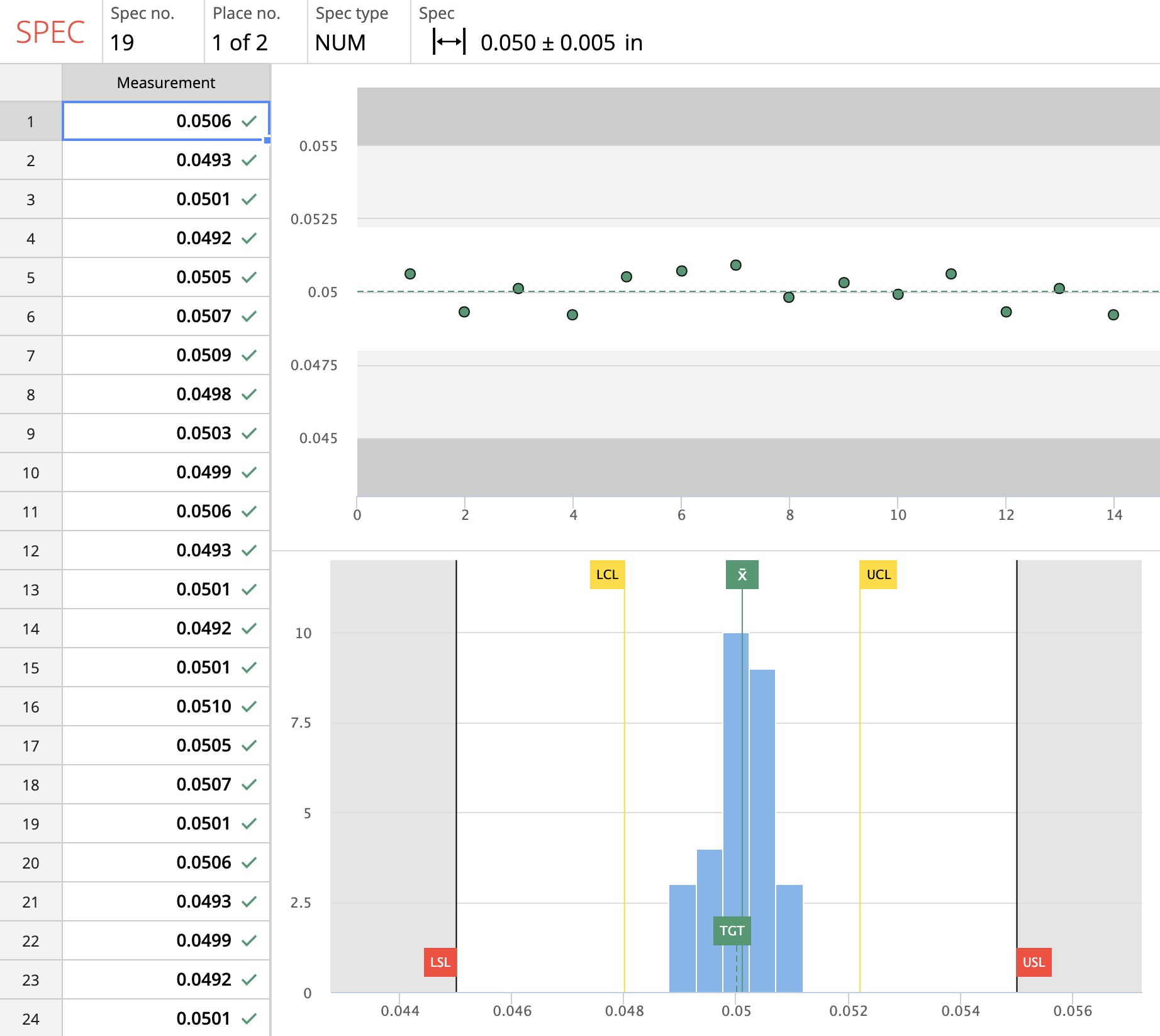
1: Plot the Data: Record the measurement data, and plot this data on a run-chart and on a histogram as shown in the picture on the right.
2: Calculate the Spec Width: Plot the Upper Spec Limit (USL) and Lower Spec Limit (LSL) on the histogram, and calculate the Spec Width as shown below.
Spec Width = USL — LSL
3: Calculate the Process Width: Similarly, we will also calculate the Process Width. The simplest way to think about the process width is "the difference between the largest value and the smallest value this process could create".
Process Width = UCL — LCL
4: Calculate Cp: Calculate the capability index as the ratio of the spec width to the process width.
Cp = Spec Width / Process Width
04. A Simple Analogy
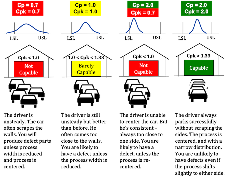
Imagine a driver trying to park a car in a garage. If the car is too wide, it won't fit. If it's narrower than the garage opening, but if it's not centered, it won't make it in - it will likely hit/scrape one of the sides. Hitting one of the sides of the garage is equivalent to producing a defective part.
But if the car is narrow enough AND well centered, the car will fit. That is our goal. We want a manufacturing process width that is narrow and well centered relative to the specification limits.

05. A More Realistic Analogy
Now let's assume that the car is the right width. It's narrow enough, and should always fit. It's now up to the driver's skill to park without scraping the sides. Imagine a driver arriving home after work each day, and parking his car in the garage.
The Good Driver: A good driver will always center the car well with enough room on both sides. Over the next 30 days, his run-chart and histogram will both be very narrow. It's clear from the charts that he's very unlikely to scrape or dent the car. There's plenty of room on either side.
The Unsteady Driver: On the other hand, an unsteady driver - someone learning to drive - may not always center the car correctly. Over the next 30 days, his run-chart and histogram are very wide. It's very likely that he could scrape or dent the car.
We'll use the same idea in manufacturing. We'll record measurements for each part made, then plot a histogram and run-chart, and see how much room we have on each side. The narrower our histogram width relative to the specification width, the higher our process capability.
06. Collecting Data
Your measurements must follow the rules below:
Gage Resolution: Gages should be calibrated and gage resolution should be at least 1/10th the specification. E.g. 0.565 +/-0.005" implies a total tolerance of 0.010, and requires a gage with resolution 0.001" or smaller.
Production Order: To calculate Cpk, parts must be measured and recorded in production order. If parts are not recorded in production order, you may miss trends and periodic fluctuations.
Record All Data: Always record data for parts that pass, as well as for parts that fail.
Ensure Traceability: Make sure all measurements are traceable back to Man (Operator), Machine (Operation), Method, Material, Measurement System, and Environmental Conditions (5Ms, 1E) to enable process improvement. Record Unit Number or Serial Number for each part.
Homogenous Data: Keep data populations separate. A change in one of the 5M, 1E values may result in non-homogenous data. For example, do not mix the measurements made with two different types of equipment (e.g. CMM, caliper) into a single data-set.
07. Process Stability
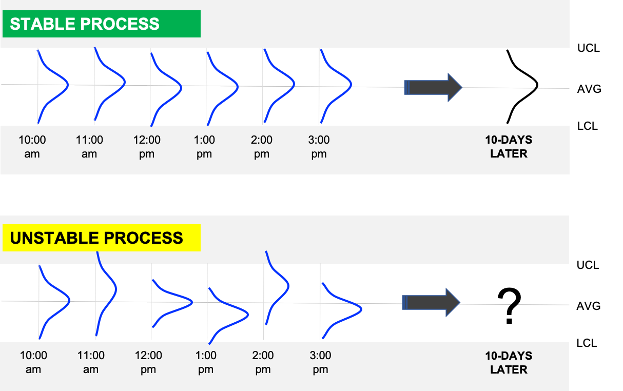
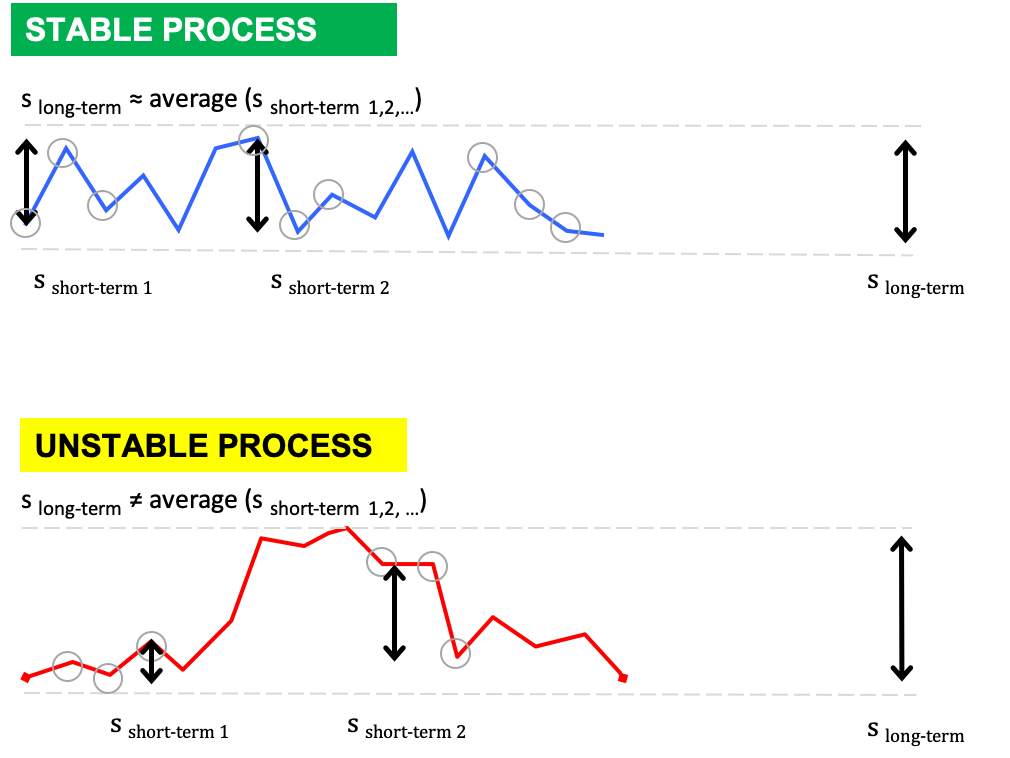
Before you begin a process capability analysis, you must check to ensure your process is stable. If your process is stable, the short-term behaviour of the process (during the initial run), will be a good predictor of the long-term behavior of the process (i.e. you can predict future performance with confidence).
Process behavior - both short-term and long-term - is characterized by the average and the standard deviation. A process will be considered stable when it's average and standard deviation are constant over time.
08. Short-Term & Long-Term Process Behaviour
For a stable process, the run chart should look relatively flat, without an upward or downward trend, and without periodic fluctuations.
Short-Term Standard Deviation:
To calculate short-term average and standard deviation, we create sub-groups of the data. Sub-groups can be created in two ways: you can either record consecutive measurements on an individuals chart and treat every two consecutive parts as a sub-group of size 2, or you can record measurements for 3 to 5 samples at a fixed interval (e.g. 5 parts every hour) on an x-bar chart.
The average and standard deviation of these sub-group measurements are called the short-term-average and short-term-standard-deviation or within-sub-group average and standard deviation.
Long-Term Standard Deviation:
Calculating long-term average and standard deviation is much simpler. We take all the measurements from the individuals charts, or from the x-bar charts, and calculate the average and standard deviation for the entire data-set.
09. Difference between Cp, Cpk and Pp, Ppk
[Potential] Process Capability Analysis (Cp, Cpk):
A process capability study uses data from a sample to PREDICT the ability of a manufacturing process to produce parts conforming to specifications. This prediction enables us to "qualify" a new manufacturing process as being fit for use in production. The index Cp provides a measure of potential process capability i.e. how well a process can perform if there is no change in the underlying process conditions.
Cpk uses "s-short-term" to predict the behavior of the process.
[Actual] Process Performance Analysis (Pp, Ppk)
A process performance study is used to EVALUATE a manufacturing process and answers the question: "how did the process actually perform over a period of time?" This is a historical analysis rather than a predictive analysis, but can still be used to drive process improvements.
Ppk uses "s-long-term" to evaluate the behavior of the process.
If the process is stable, Ppk = Cpk, i.e. the actual performance will match the predicted potential performance. However, if the process is unstable &emdash; i.e. if it shifts or drifts over time &emdash; you will find Ppk << Cpk.
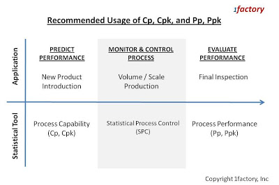
10. Difference between Process Capability and Statistical Process Control
SPC is a tool for monitoring and controlling a production process to prevent the production of non-conforming product. The key term here is "control".
Unlike Process Capability and Process Performance Analyses where we measure and analyze without changing settings until after the study is complete, SPC requires that we measure, analyze, and act on the analysis real time.
SPC helps us detect instability in the process due to things like tool wear, a drop in clamp pressure etc, and therefore requires that we make the necessary adjustments to ensure that the process is returned to stability and continues to produce parts within specifications.
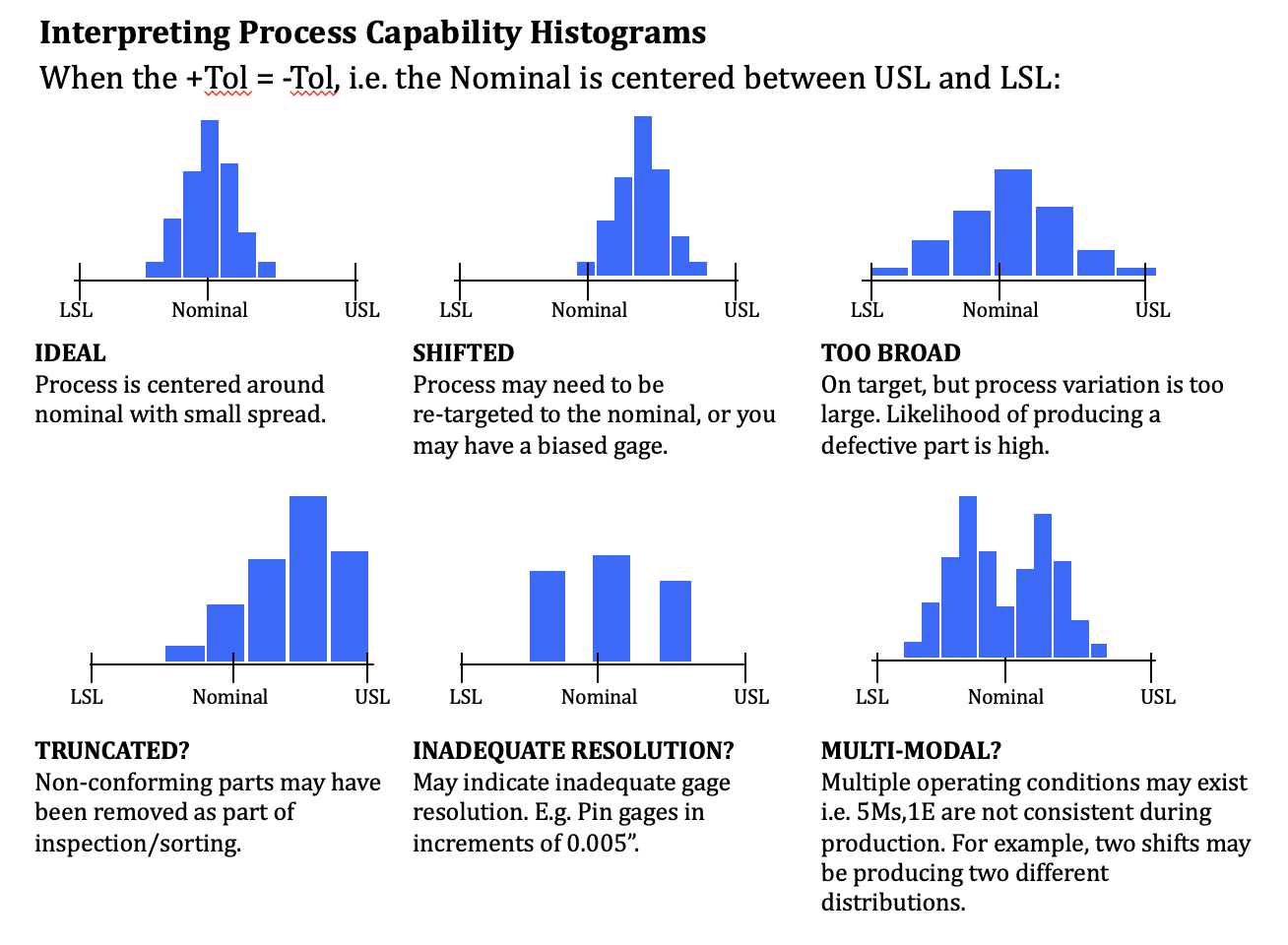
11. Interpreting Process Capability Histograms
The histograms on the right, show various commonly encountered use cases.
Ideal: In the ideal case, your process is centered over the Nominal, with a narrow distribution, leaving plenty of white space to the LSL and USL. You are unlikely to produce defective parts even if the process starts to drift.
Shifted: If the process is shifted towards either the LSL or the USL, a small shift in the process could result in a defect.
Too Broad: If the process is too broad, a small shift in the process, towards either the LSL or USL, could result in a defect.
Truncated: A truncated distribution may indicate that out-of-spec parts have been removed from the data set.
Inadequate Resolution: Inadequate gage resolution may result in misleading calculations of the average and standard deviation.
Multi-Modal: A distribution with more than one peak may be caused by multiple operating conditions. E.g. data from two different mold cavities, production from two very different machines etc.
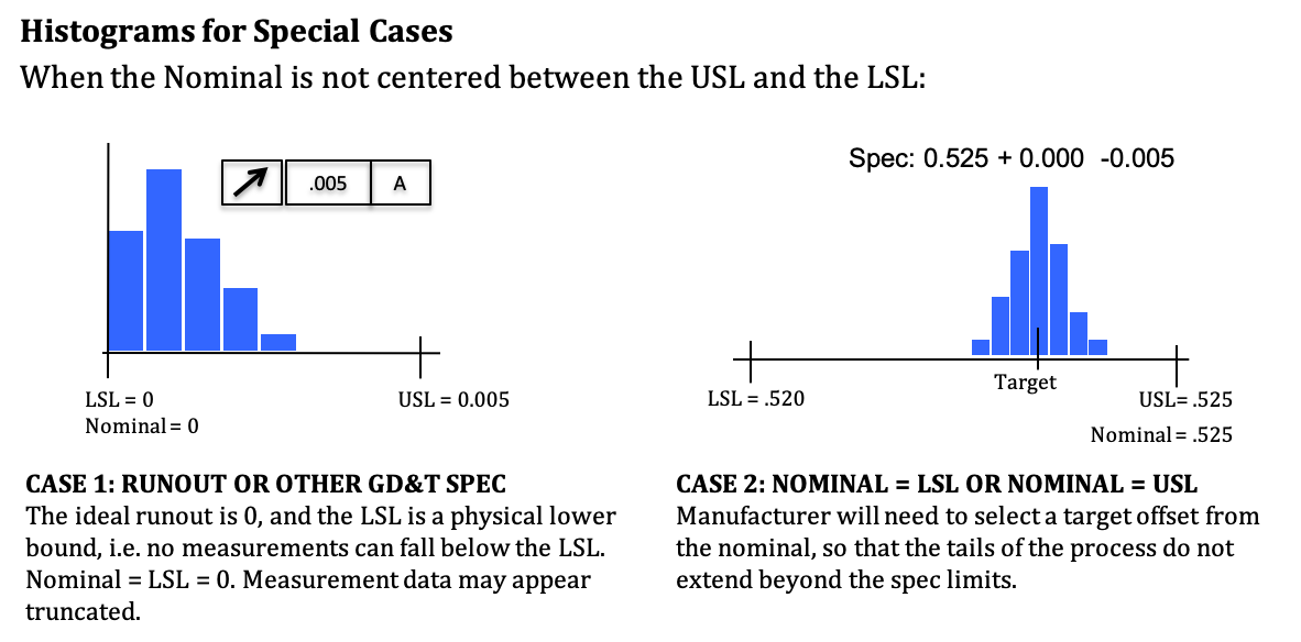
12. Histograms for Special Cases
GD&T: For most Geometric dimensions, the ideal value is 0, and the LSL is a physical lower bound, i.e. no measurements can fall below the LSL. In other words, the Nominal = LSL = 0. The ideal measurements therefore will be exactly at or close to the LSL, and in this particular case, we do want measurements to be close to the LSL.
Unilateral Specs: Making parts at the nominal will be too risky. The manufacturing engineer will therefore need to select a target value offset from the nominal, so that the tails of the process do not extend beyond the spec limits.
13. What Cpk Value Should You Aim For?
In general, the higher the Cpk, the better. A Cpk value less than 1.0 is considered poor and the process is not capable. A value between 1.0 and 1.33 is considered barely capable, and a value greater than 1.33 is considered capable.
But, you should aim for a Cpk value of 2.00 or higher where possible. A Cpk of 2.00 implies that the process uses only 50% of the spec width, significantly reducing the risk of defect.
A high Cpk value has two important benefits:
(1) You'll be producing fewer defective parts
(2) You'll improve your product's performance
The second benefit may not be very obvious. Watch a video here to see how a Cpk (or Ppk) of 4.00 i.e. using only 25% of the spec width, resulted in significantly better product performance for an automotive transmission manufacturer, with 75% fewer warranty complaints.
14. Automating Cp, Cpk, and Pp, Ppk Calculations
1factory's Manufacturing Quality Control software automatically calculates Process Capability (Cp, Cpk, Cpl, Cpu) and Process Performance (Pp, Ppk, Ppl, Ppu) for each production lot and across lots saving hours of time. Learn More